ANt Collony Algorithm

REFRENSI ANT:

XY =

    82    66
    91     3
    12    85
    92    94
    63    68
     9    76
    28    75
    55    39
    96    66
    97    17
    15    71
    98     3
    96    27
    49     4
    80     9
    14    83
    42    70
    92    32
    80    95
    96     3

Sistem akan auto move mencari jarak terdekat untuk melalui semua titik yang ada..

dan ini adalah grafik kecerdasannya...
Iteration 1: Best Cost = 650.2307
Iteration 2: Best Cost = 540.892
Iteration 3: Best Cost = 531.4992
Iteration 4: Best Cost = 483.6564
Iteration 5: Best Cost = 483.6564
Iteration 6: Best Cost = 483.6564
Iteration 7: Best Cost = 483.6564
Iteration 8: Best Cost = 451.971
Iteration 9: Best Cost = 451.9041
Iteration 10: Best Cost = 439.1259
Iteration 11: Best Cost = 439.1259
Iteration 12: Best Cost = 424.478
Iteration 13: Best Cost = 424.478
Iteration 14: Best Cost = 410.1005
Iteration 15: Best Cost = 410.1005
Iteration 16: Best Cost = 410.1005
Iteration 17: Best Cost = 410.1005
Iteration 18: Best Cost = 410.1005
Iteration 19: Best Cost = 410.1005
Iteration 20: Best Cost = 410.1005

Code Aplikasi.m:

model=CreateModel();
CostFunction=@(tour) TourLength(tour,model);

nVar=model.n;
MaxIt=20;      % Maximum Number of Iterations
nAnt=40;        % Number of Ants (Population Size)
Q=1;
tau0=10*Q/(nVar*mean(model.D(:))); % Initial Phromone

alpha=1;        % Phromone Exponential Weight
beta=1;         % Heuristic Exponential Weight

rho=0.05;       % Evaporation Rate

eta=1./model.D;             % Heuristic Information Matrix
tau=tau0*ones(nVar,nVar);   % Phromone Matrix
BestCost=zeros(MaxIt,1);    % Array to Hold Best Cost Values

empty_ant.Tour=[];empty_ant.Cost=[];

ant=repmat(empty_ant,nAnt,1);
BestSol.Cost=inf;

for it=1:MaxIt 
    for k=1:nAnt 
        ant(k).Tour=randi([1 nVar]);
     
        for l=2:nVar
            i=ant(k).Tour(end);
            P=tau(i,:).^alpha.*eta(i,:).^beta;
            P(ant(k).Tour)=0;
            P=P/sum(P);
            j=RouletteWheelSelection(P);
            ant(k).Tour=[ant(k).Tour j];   
        end
        ant(k).Cost=CostFunction(ant(k).Tour);
        if ant(k).Cost<BestSol.Cost
            BestSol=ant(k);
        end
     
    end
 
    % Update Phromones
    for k=1:nAnt
        tour=ant(k).Tour;
        tour=[tour tour(1)];
        for l=1:nVar
            i=tour(l);
            j=tour(l+1);
            tau(i,j)=tau(i,j)+Q/ant(k).Cost;
        end
    end
 
 
    tau=(1-rho)*tau;
    % Store Best Cost
    BestCost(it)=BestSol.Cost;
 
    % Show Iteration Information
    disp(['Iteration ' num2str(it) ': Best Cost = ' num2str(BestCost(it))]);
 
    % Plot Solution
    figure(1);
    PlotSolution(BestSol.Tour,model);
    pause(2);%0.01
 
end

%% Results
figure;
plot(BestCost,'LineWidth',2);
xlabel('Iteration');
ylabel('Best Cost');
grid on;

++++++++++++++++++++++++

function model=CreateModel()

    x=[82 91 12 92 63 9 28 55 96 97 15 98 96 49 80 14 42 92 80 96];

    

    y=[66 3 85 94 68 76 75 39 66 17 71 3 27 4 9 83 70 32 95 3];

    

    n=numel(x);

    

    D=zeros(n,n);

    

    for i=1:n-1

        for j=i+1:n

            

            D(i,j)=sqrt((x(i)-x(j))^2+(y(i)-y(j))^2);

            

            D(j,i)=D(i,j);

            

        end

    end

    

    model.n=n;

    model.x=x;

    model.y=y;

    model.D=D;

end

++++++++++++++++++++++++++++++++++++

function L=TourLength(tour,model)

    n=numel(tour);

    tour=[tour tour(1)];

    

    L=0;

    for i=1:n

        L=L+model.D(tour(i),tour(i+1));

    end

end

++++++++++++++++++++++++++++++++++++++

function j=RouletteWheelSelection(P)

    r=rand;

    

    C=cumsum(P);

    

    j=find(r<=C,1,'first');

end

++++++++++++++++++++++++++++++++++++++

function PlotSolution(tour,model)

    tour=[tour tour(1)];

    

    plot(model.x(tour),model.y(tour),'k-o',...

        'MarkerSize',10,...

        'MarkerFaceColor','y',...

        'LineWidth',1.5);

    

    xlabel('x');

    ylabel('y');

    

    axis equal;

    grid on;

    

alpha = 0.1;

    xmin = min(model.x);

    xmax = max(model.x);

    dx = xmax - xmin;

    xmin = floor((xmin - alpha*dx)/10)*10;

    xmax = ceil((xmax + alpha*dx)/10)*10;

    xlim([xmin xmax]);

    

    ymin = min(model.y);

    ymax = max(model.y);

    dy = ymax - ymin;

    ymin = floor((ymin - alpha*dy)/10)*10;

    ymax = ceil((ymax + alpha*dy)/10)*10;

    ylim([ymin ymax]);

    

    

end

++++++++++++++++++++++++++++++++++++++++

GB Phromone 

+++++++++++++++++++++++++++++++++++++++++++++++++++

GB BestRute

+++++++++++++++++++++++++++++++++++++++++++++++++++

SImple Image Processing

https://www.mathworks.com/campaigns/offers/image-segmentation.confirmation.html?s_iid=ans_image-segmentation_370902_rcspot&ab_test=b_version

https://www.mathworks.com/content/dam/mathworks/tag-team/Objects/d/88390_93007v00_Detecting_Cell_Image_Segmentation_2016.pdf


https://www.mathworks.com/matlabcentral/fileexchange/48859-segment-images-interactively-and-generate-matlab-code?s_tid=res_ip_kit3


https://www.mathworks.com/content/dam/mathworks/tag-team/Objects/d/88370_93003v00-detecting-meas-circular-obj-image-2016.pdf


https://www.mathworks.com/content/dam/mathworks/tag-team/Objects/p/88395_93008v00_Texture_Gabor_Filters_2016.pdf

https://www.mathworks.com/help/images/identifying-round-objects.html

Image imfill 'holes' Dan BoundingBox

J = imread('img3.png');
I = rgb2gray(J);
% imshow(I), title('image original grisé');
[~, threshold] = edge(I, 'sobel');
fudgeFactor = .5;
BWs = edge(I,'sobel', threshold * fudgeFactor);
figure, imshow(BWs), title('binary gradient mask');
se90 = strel('line', 3, 90);
se0 = strel('line', 3, 0);
BWsdil = imdilate(BWs, [se90 se0]);
figure, imshow(BWsdil), title('dilated gradient mask');
BWdfill = imfill(BWsdil, 'holes');
figure, imshow(BWdfill);
title('binary image with filled holes');
BWnobord = imclearborder(BWdfill, 4);
figure, imshow(BWnobord), title('cleared border image');
seD = strel('diamond',1);
BWfinal = imerode(BWnobord,seD);
BWfinal = imerode(BWfinal,seD);
figure, imshow(BWfinal), title('segmented image');
BWoutline = bwperim(BWfinal);
Segout = J;
Segout(BWoutline) = 255;
figure,
imshow(Segout), title('outlined original image');

OK


hold on;
labeledImage =BWoutline; %not needed, image should be already in logical
measurements = regionprops(labeledImage, 'BoundingBox');
for k = 1 : length(measurements)
    thisBB = measurements(k).BoundingBox;
    rectangle('Position',[thisBB(1),thisBB(2),thisBB(3),thisBB(4)],'EdgeColor','b','LineWidth',1 );
end

Jika Ingin Langusng di Crop saja objek yang sudah ditemukan tsb:

grayImage = BWoutline;
% Display the image.
imshow(grayImage);
S = regionprops(grayImage,'BoundingBox','Area');
[MaxArea,MaxIndex] = max(vertcat(S.Area));
imshow(grayImage,'InitialMagnification',20)
%// Highlight the required object
hold on
rectangle('Position',S(MaxIndex).BoundingBox,'LineWidth',2,'EdgeColor','y')
Length = S(MaxIndex).BoundingBox(3);
Height = S(MaxIndex).BoundingBox(4);
% Cropping the image
% Get all rows and columns where the image is nonzero
[nonZeroRows,nonZeroColumns] = find(grayImage);
% Get the cropping parameters
topRow = min(nonZeroRows(:));
bottomRow = max(nonZeroRows(:));
leftColumn = min(nonZeroColumns(:));
rightColumn = max(nonZeroColumns(:));
% Extract a cropped image from the original.
croppedImage = grayImage(topRow:bottomRow, leftColumn:rightColumn);
% Display the original gray scale image.
figure
imshow(croppedImage, []);

AutoCrop regionProp

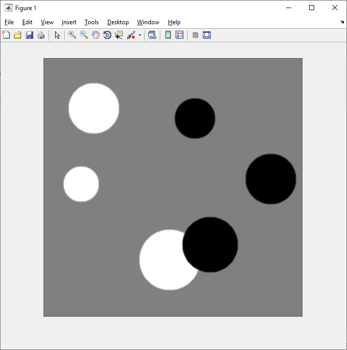
 a = imread('circlesBrightDark.png');
          bw = a > 200;
          imshow(bw)
          title('Image with Circles')

          stats = regionprops('table',bw,'Centroid','MajorAxisLength','MinorAxisLength','BoundingBox');%,'BoundingBox'
           M=stats.BoundingBox;

  mask2=M(3,:);
        croppedImage = imcrop(bw, mask2);
        figure,imshow(croppedImage);title('Cropped Image');

M =

   40.5000  215.5000   69.0000   69.0000
   50.5000   50.5000   99.0000   99.0000
  190.5000  340.5000  115.0000  119.0000

Atau mau seperti ini hasilnya : PAKAI CENTROID


stats =

  3×4 table

        Centroid        BoundingBox     MajorAxisLength    MinorAxisLength
    ________________    ____________    _______________    _______________

        75       250    [1x4 double]    70.016             70.016       
       100       100    [1x4 double]    99.924             99.924       
    242.94    402.67    [1x4 double]    126.23             101.54     


 a = imread('circlesBrightDark.png');
          bw = a > 200;
          imshow(bw)
          title('Image with Circles')
 
          stats = regionprops('table',bw,'Centroid','MajorAxisLength','MinorAxisLength','BoundingBox');%,'BoundingBox'
          centers = stats.Centroid;
          diameters = mean([stats.MajorAxisLength stats.MinorAxisLength],2);
          radii = diameters/2;
 
          % Plot the circles
          hold on
          viscircles(centers,radii);
          hold off
         
++++++++++++++++++++++++

RGB = imread('pillsetc.png');
%imshow(RGB)
I = rgb2gray(RGB);
bw = imbinarize(I);%logical
    %imshow(bw)
    % bw = bwareaopen(bw,30); %logical +NR
    % %imshow(bw)
    % se = strel('disk',2);
    % bw = imclose(bw,se);%logical
    %imshow(bw) 

bw = imfill(bw,'holes');%logical +Fill
imshow(bw)
stats = regionprops('table',bw,'Centroid','MajorAxisLength','MinorAxisLength','BoundingBox');
M=stats.BoundingBox;
hold on
for k = 1:length(M)
    N = M(k,:)
    rectangle('Position',N,'FaceColor','r')
end

+++++++++++++++++++++++++++++

RGB = imread('pillsetc.png');
%imshow(RGB)
I = rgb2gray(RGB);
bw = imbinarize(I);%logical
    %imshow(bw)
    % bw = bwareaopen(bw,30); %logical +NR
    % %imshow(bw)
    % se = strel('disk',2);
    % bw = imclose(bw,se);%logical
    %imshow(bw) 

bw = imfill(bw,'holes');%logical +Fill
imshow(bw)

[B,L] = bwboundaries(bw,'noholes');

imshow(label2rgb(L,@jet,[.5 .5 .5]))

hold on

for k = 1:length(B)

  boundary = B{k};

  plot(boundary(:,2),boundary(:,1),'w','LineWidth',2);

end

+++++++++++++++++++++++++++++++++++++++++++

stats = regionprops(L,'Area','Centroid');

threshold = 0.94;

for k = 1:length(B)

  % obtain (X,Y) boundary coordinates corresponding to label 'k'

  boundary = B{k};

  % compute a simple estimate of the object's perimeter

  delta_sq = diff(boundary).^2;    

  perimeter = sum(sqrt(sum(delta_sq,2)));

  

  % obtain the area calculation corresponding to label 'k'

  area = stats(k).Area;

  

  % compute the roundness metric

  metric = 4*pi*area/perimeter^2;

  

  % display the results

  metric_string = sprintf('%2.2f',metric);

  % mark objects above the threshold with a black circle

  if metric > threshold

    centroid = stats(k).Centroid;

    plot(centroid(1),centroid(2),'ko');

  end

  

 text(boundary(1,2)-35,boundary(1,1)+13,metric_string,'Color','y','FontSize',14,'FontWeight','bold')

  

end

title(['Metrics closer to 1 indicate that ',  'the object is approximately round'])

Analisa Jenis Kucing sebaiknya pakai ViolaJones

hasil Akurasi:
  'OUTPUT'    'PREDIKSI1'    'T/F'    'PREDIKSI2'    'T/F'
     1     7     0     1     1
     1     7     0     1     1
     1     7     0     1     1
     1     7     0     1     1
     1     7     0     1     1
     2     2     1     2     1
     2     2     1     2     1
     2     2     1     2     1
     2     2     1     2     1
     2     2     1     2     1
     3     3     1     3     1
     3     3     1     3     1
     3     3     1     3     1
     3     3     1     3     1
     3     3     1     3     1
     4     4     1     4     1
     4     4     1     4     1
     4     4     1     4     1
     4     4     1     4     1
     4     4     1     4     1
     5     5     1     5     1
     5     5     1     5     1
     5     5     1     5     1
     5     5     1     5     1
     5     5     1     5     1
     6     6     1     6     1
     6     6     1     6     1
     6     6     1     6     1
     6     6     1     6     1
     6     6     1     6     1
     7     7     1     7     1
     7     7     1     7     1
     7     7     1     7     1
     7     7     1     7     1
     7     7     1     7     1

output adalah terget yang harus di capai...

misal 1: kucing Angora, 2 Kucing Bengal, 3 Brits, 4 Exotic, 5 Mainecoon, 6 Persia dan  7 Sphynx

Menggunakan Metode SVM model Grayscale (rgb2gray): hasilnya kurang baik

Menggunakan Metode SVM model R+G/2(Red dan green saja): hasilnya lebih baik bahkan 100% benar

'T/F' =>1=true, 2 false atau tidak sesuai target 

Saat menggunakan Kmeans hasilya kurang baik karena disini menggunakan rumus labeling....

pil1=get(handles.pil1,'Userdata')
pil2=get(handles.pil2,'Userdata')
pil3=get(handles.pil3,'Userdata')
pil4=get(handles.pil4,'Userdata')


data=get(handles.mytable3,'Userdata');
data0=get(handles.mytable4,'Userdata');

if size(data,1)<1
   msgbox('Silakan pilih data latih dahhulu...','Lengkapi Data','help');
    return;
end

ROW=data(:,1)

co=size(data0,2);
mydata=data0(:,2:co);
mydatabaru=[pil1,pil2,pil3,pil4]
F=[mydata;mydatabaru];

K=8;
opts = statset('Display','final');
[prediction, CENTS] = kmeans(F, K, 'Distance','city','Replicates',40, 'Options',opts);

header=["X1","X2","X3","X4"];
c=size(CENTS,1);

T=size(prediction,1);
hsl=prediction(T);
row=linspace(1,c,c);
set(handles.mytable5,'data',CENTS,'ColumnName',header,'RowName',row);
set(handles.mytable5,'Userdata',CENTS);
OUT=cell2mat(ROW(hsl));
set(handles.edknn,'String',num2str(OUT));

+++++++++++++++++++

Perhitungan Normalsiasi SVM menggunalan rumus ini:

load DLATIH.mat;

load DLATIH2.mat;

load ROW.mat;

load ROW2.mat;

load KAT.mat;

kolom={'Contrast' 'Correlation' 'Energy' 'Homogeneity'};

    

set(handles.mytable,'data',DLATIH,'ColumnName',kolom,'RowName',ROW);

set(handles.mytable,'Userdata',DLATIH); 

%%%%%%%%%%%%%%%

set(handles.mytable2,'data',DLATIH2,'ColumnName',kolom,'RowName',ROW);

set(handles.mytable2,'Userdata',DLATIH2); 

%%%%%%%%%%%%%%%

  

   

%%%%%%%%%%%%%%%%%%%%

X =DLATIH;

Y = KAT;

prediction=multisvm(DLATIH,KAT,DLATIH);

prediction2=prediction';

ba=size(prediction2,2);

benar=0;

rekap1=[];

for i=1:ba

    if(KAT(1,i)==prediction2(1,i))

       benar=benar+1; 

       rekap1(1,i)=1;

    else

        rekap1(1,i)=0;

    end

end  

salah=ba-benar;

akurasi1=benar/ba;

prediction=multisvm(DLATIH2,KAT,DLATIH2);

prediction22=prediction';

ba=size(prediction22,2);

benar=0;

rekap2=[];

for i=1:ba

    if(KAT(1,i)==prediction22(1,i))

       benar=benar+1;

       rekap2(1,i)=1;

    else

        rekap2(1,i)=0;

    end

end  

salah=ba-benar;

akurasi2=benar/ba;

GAB=[KAT' prediction2' rekap1'  prediction22' rekap2']

row=linspace(1,ba,ba);

header={'OUTPUT','PREDIKSI1','T/F','PREDIKSI2','T/F'}

set(handles.mytable0,'data',GAB,'ColumnName',header,'RowName',row);

set(handles.mytable0,'Userdata',GAB);

Sedang raget yang hendak dicapai lebihd ari 2 item maka menggunakan rumsu Multisvm sbb:

function [itrfin] = multisvm( T,C,test )

itrind=size(test,1);

itrfin=[];

Cb=C;

Tb=T;

for tempind=1:itrind

    tst=test(tempind,:);

    C=Cb;

    T=Tb;

    u=unique(C);

    N=length(u);

    c4=[];

    c3=[];

    j=1;

    k=1;

    if(N>2)

        itr=1;

        classes=0;

        cond=max(C)-min(C);

        while((classes~=1)&&(itr<=length(u))&& size(C,2)>1 && cond>0)

            c1=(C==u(itr));

            newClass=c1;

            svmStruct = svmtrain(T,newClass,'kernel_function','polynomial');  

            classes = svmclassify(svmStruct,tst);

            

            for i=1:size(newClass,2)

                if newClass(1,i)==0;

                    c3(k,:)=T(i,:);

                    k=k+1;

                end

            end

            T=c3;

            c3=[];

            k=1;

            

            for i=1:size(newClass,2)

                if newClass(1,i)==0;

                    c4(1,j)=C(1,i);

                    j=j+1;

                end

            end

            C=c4;

            c4=[];

            j=1;

            

            cond=max(C)-min(C); 

            if classes~=1

                itr=itr+1;

            end

        end

    end

    

    valt=Cb==u(itr);

    val=Cb(valt==1);

    val=unique(val);

    itrfin(tempind,:)=val;

end

end

Datalatih target:


    'Anggora'
    'Anggora'
    'Anggora'
    'Anggora'
    'Anggora'
    'Bengal'
    'Bengal'
    'Bengal'
    'Bengal'
    'Bengal'
    'Britsh'
    'Britsh'
    'Britsh'
    'Britsh'
    'Britsh'
    'Exotic'
    'Exotic'
    'Exotic'
    'Exotic'
    'Exotic'
    'Mainecoon'
    'Mainecoon'
    'Mainecoon'
    'Mainecoon'
    'Mainecoon'
    'Persia'
    'Persia'
    'Persia'
    'Persia'
    'Persia'
    'Sphynx'
    'Sphynx'
    'Sphynx'
    'Sphynx'
    'Sphynx'

DLATIH =

   1.0e+10 *

    0.1114    1.0030    0.0106    0.0000
    0.1114    1.0030    0.0106    0.0000
    0.1114    1.0030    0.0106    0.0000
    0.0959    1.0573    0.0153    0.0000
    0.1114    1.0030    0.0106    0.0000
    0.1276    2.5270    0.0104    0.0000
    0.1276    2.5270    0.0104    0.0000
    0.1276    2.5270    0.0104    0.0000
    0.1276    2.5270    0.0104    0.0000
    0.1276    2.5270    0.0104    0.0000
    0.0669    0.6027    0.0046    0.0000
    0.0669    0.6027    0.0046    0.0000
    0.0669    0.6027    0.0046    0.0000
    0.0669    0.6027    0.0046    0.0000
    0.0669    0.6027    0.0046    0.0000
    0.0893    0.2997    0.0045    0.0000
    0.0893    0.2997    0.0045    0.0000
    0.0893    0.2997    0.0045    0.0000
    0.0893    0.2997    0.0045    0.0000
    0.0893    0.2997    0.0045    0.0000
    0.1419    3.0747    0.0114    0.0000
    0.0732    1.1291    0.0145    0.0000
    0.1418    1.8808    0.0081    0.0000
    0.0892    1.3324    0.0200    0.0000
    0.1418    0.9196    0.0120    0.0000
    0.1114    0.8824    0.0063    0.0000
    0.1114    0.8824    0.0063    0.0000
    0.1114    0.8824    0.0063    0.0000
    0.1114    0.8824    0.0063    0.0000
    0.1421    1.1542    0.0027    0.0000
    0.1099    1.0015    0.0114    0.0000
    0.1099    1.0015    0.0114    0.0000
    0.1099    1.0015    0.0114    0.0000
    0.1099    1.0015    0.0114    0.0000
    0.1099    1.0015    0.0114    0.0000

>> DLATIH2

DLATIH2 =

   1.0e+10 *

    0.1114    1.0030    0.0106    0.0000
    0.1114    1.0030    0.0106    0.0000
    0.1114    1.0030    0.0106    0.0000
    0.0959    1.0573    0.0153    0.0000
    0.1114    1.0030    0.0106    0.0000
    0.1276    2.5270    0.0104    0.0000
    0.1276    2.5270    0.0104    0.0000
    0.1276    2.5270    0.0104    0.0000
    0.1276    2.5270    0.0104    0.0000
    0.1276    2.5270    0.0104    0.0000
    0.0669    0.6027    0.0046    0.0000
    0.0669    0.6027    0.0046    0.0000
    0.0669    0.6027    0.0046    0.0000
    0.0669    0.6027    0.0046    0.0000
    0.0669    0.6027    0.0046    0.0000
    0.0893    0.2997    0.0045    0.0000
    0.0893    0.2997    0.0045    0.0000
    0.0893    0.2997    0.0045    0.0000
    0.0893    0.2997    0.0045    0.0000
    0.0893    0.2997    0.0045    0.0000
    0.1419    3.0747    0.0114    0.0000
    0.0732    1.1291    0.0145    0.0000
    0.1418    1.8808    0.0081    0.0000
    0.0892    1.3324    0.0200    0.0000
    0.1418    0.9196    0.0120    0.0000
    0.1114    0.8824    0.0063    0.0000
    0.1114    0.8824    0.0063    0.0000
    0.1114    0.8824    0.0063    0.0000
    0.1114    0.8824    0.0063    0.0000
    0.1421    1.1542    0.0027    0.0000
    0.1099    1.0015    0.0114    0.0000
    0.1099    1.0015    0.0114    0.0000
    0.1099    1.0015    0.0114    0.0000
    0.1099    1.0015    0.0114    0.0000
    0.1099    1.0015    0.0114    0.0000


Terlihat 0 tetapi sebanarnya nilainya ada......cb di lihat lebih detail:
>> DLATIH2(1,4)

ans =

   1.6878e+04

Pengolahan Data AUDIO

Cara mendeteksi Suara Audio itu masuk kategori apa yaaaa?

SKhirnya bisa di buktikan bahwa Konsep audio juga semudah konsep Image bahwa mudah juga selama kita bisa menormalsiasikana sinyal audio tsresbut ...
Contoh di atas menunjukkan proses2nya
Dengan menggunakan 2 metode KNN dan SVM didapat akurasi yang baik juga

Namun begitu...SVM lebih baik akurasinyaaaa...tahu kenapaa......jelas karena ia mampu mengenali fitur objek audio dengan sempurna daripada hanya sebatas menghitung jarak menggunakan KNN

dan ini adalah sinyal normalisasi dari Audio musik nya (Gambang dan Tehyan)

Untuk Normalisasi nya rekan2 silakan bisa gunakan MFCC dengan code sbb:


function [ mfcc_test,ww ] = getMFCC( Samples)
% [InputIn,fs]=audioread(path);
% Samples = InputIn;
zz = find(Samples) < max(Samples/3);%Threshold speech regions
Samples(zz) = 0;
zz = find(Samples);
Speech_Region = Samples(zz);  

OverlapSize = 0.5;
MFCCNo = 45;
NoOfWindows = 25;
NoOfFilters = floor(MFCCNo/NoOfWindows+1);

mfcc_test = zeros(1,MFCCNo);
WindowSize = floor((size(Speech_Region,1))/(NoOfWindows+1));
ww = 0;
for ll = 0:OverlapSize:(NoOfWindows-1)/2
    bb = Speech_Region(floor(ll*WindowSize)+1:floor(ll*WindowSize)+WindowSize).*hamming(WindowSize);
    fb = fft(bb);                
    mb = 2595 * log10(1 + fb./700);                
    mfout = dct(log(abs(mb)),NoOfFilters);                    
    mfcc_test(1,ww*NoOfFilters+1:ww*NoOfFilters+NoOfFilters) = mfout;                                                        
    ww = ww + 1;
end          

end

KMEANS EXAMPLE

clc
clear all
close all
%% Generate Points
Sigma = [0.5 0.05; 0.05 0.5];
f1    = mvnrnd([0.5 0]  ,Sigma,100);
f2    = mvnrnd([0.5 0.5],Sigma,100);
f3    = mvnrnd([0.5 1]  ,Sigma,100);
f4    = mvnrnd([0.5 1.5],Sigma,100);
F     = [f1;f2;f3;f4];
%% K-means
K     = 8;                                            % Cluster Numbers
KMI   = 40;                                           % K-means Iteration
CENTS = F( ceil(rand(K,1)*size(F,1)) ,:);             % Cluster Centers
DAL   = zeros(size(F,1),K+2);                         % Distances and Labels
CV    = '+r+b+c+m+k+yorobocomokoysrsbscsmsksy';       % Color Vector
for n = 1:KMI
       
   for i = 1:size(F,1)
      for j = 1:K 
        DAL(i,j) = norm(F(i,:) - CENTS(j,:));     
      end
      [Distance CN] = min(DAL(i,1:K));                % 1:K are Distance from Cluster Centers 1:K
      DAL(i,K+1) = CN;                                % K+1 is Cluster Label
      DAL(i,K+2) = Distance;                          % K+2 is Minimum Distance
   end
   for i = 1:K
      A = (DAL(:,K+1) == i);                          % Cluster K Points
      CENTS(i,:) = mean(F(A,:));                      % New Cluster Centers
      if sum(isnan(CENTS(:))) ~= 0                    % If CENTS(i,:) Is Nan Then Replace It With Random Point
         NC = find(isnan(CENTS(:,1)) == 1);           % Find Nan Centers
         for Ind = 1:size(NC,1)
         CENTS(NC(Ind),:) = F(randi(size(F,1)),:);
         end
      end
   end
 
%% Plot 
clf
figure(1)
hold on
 for i = 1:K
PT = F(DAL(:,K+1) == i,:);                            % Find points of each cluster   
plot(PT(:,1),PT(:,2),CV(2*i-1:2*i),'LineWidth',2);    % Plot points with determined color and shape
plot(CENTS(:,1),CENTS(:,2),'*k','LineWidth',7);       % Plot cluster centers
 end
hold off
grid on
pause(0.1)
end